home..

Explainable Scores For Randomized Tree Ensembles

Dingyi Lai / August 2022

Introduction

Starting from a general question: How to explain the prediction from a machine learning black-box algorithm?

This blog will guide you through the general defintion of Explainable AI (XAI), the mainstream methods used in general, and then focus specifically on tree-based models. Finally, we compare two methods on some open dataset. The ideas presented here draw heavily on my collaboration with Prof. Dr. Markus Loecher, with the primary references being the paper Approximation of SHAP Values for Randomized Tree Ensembles and Markus’s blog: CFC-SHAP Visualization.

Explainable AI (XAI)

I was introduced to this topic in a machine learning course at TU Berlin, where it was defined as understanding how a machine learning model produces its prediction – that is, which features it uses, how they are combined, and to what input pattern the model responds most strongly.

One global XAI method is activation maximization, where we generate the samples that maximally activates a specific output neuron or class. For instance, by choosing a regularizer such as the log likelihood of observations $x$, we compute the typical input $x^*$ that maximize the sum of a log-probablity for a specific class and the regularizer:

\[x^* = \arg\max_{x} \{ \log p(\omega_c \mid x) + \log p(x) \} = \arg\max_{x} \log p(x \mid \omega_c)\]

However, this method does not provide feature-level attribution to a single prediction. Figure 1 (below) conceptually illustrates the need for local explanations.

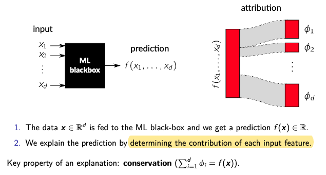
Conceptual table — Figure 1: Local Explainable Score of a Prediction for Input Feature$$d$$

Commonly Used Explainable Scores

SHAP (SHapley Additive exPlanations)

SHAP values have their origins in game theory (Shapley, 1951), where they assign payoffs to players in a cooperative game. In machine learning, each input feature is treated as a player, and the prediction is the collective profit. SHAP computes the average marginal contribution of a feature over all possible feature orderings.

Pros:

Strong theoretical foundations, satisfying properties such as local accuracy, consistency, and missingness.
Provides both local (per instance) and global (model-wide) explanations.

Cons:

Computationally challenging for high-dimensional data.

The SHAP value for the $i$-th feature is defined as:

\[\phi_{i}(f,x) = \sum_{r \in R} \frac{1}{M!} \left[ f_{x}(P^{r}_{i} \cup \{i\}) - f_{x}(P^{r}_{i}) \right]\]

where:

$R$: Set of all possible feature orderings,
$P^{r}_{i}$: Set of features that come before feature $i$ in ordering $r$,
$M$: Total number of input features,
$f_{x}(S)$: Conditional expectation of the model output given the feature subset $S$.

For code examples on computing SHAP values with tree models, please refer to Markus’s blog on CFC-SHAP Visualization.

Conditional feature contributions (CFCs)

CFCs (also known as Saabas values) provide explanations by quantifying the node-wise reduction in a loss function along a decision path in a tree. They compute a weighted average of the contribution differences over all nodes that split on a particular feature.

Pros:

Efficient computation compared to full SHAP.
Offers intuitive, local explanations by directly following a tree’s decision path.
Cons:
May exhibit bias in local explanations when features at the tree’s root are undervalued.
Lacks some theoretical guarantees, such as consistency, that are inherent to SHAP values.

For the $i$-th feature, the CFC (Saabas value) is defined as:

\[\phi^{s}_{i}(f,x) = \sum_{j \in D^{i}_{x}} \left[ f_{x}(A_{j} \cup \{j\}) - f_{x}(A_{j}) \right]\]

where:

$D^{i}_{x}$: Set of nodes on the decision path for instance $x$ that split on feature $i$,
$A_{j}$: Set of features split on by the ancestors of node $j$,
$f_{x}(S)$: Estimated expectation of the model output conditioned on the set $S$ of feature values.

Approximation of SHAP Values for Randomized Tree Ensembles

Randomized tree ensembles—such as random forests and gradient boosted trees—combine multiple decision trees to improve predictive performance and stability. By introducing randomness (e.g., via bootstrapping or random feature selection), these ensembles reduce overfitting and enhance generalization. Both SHAP and CFC methods are applied to these ensembles to interpret the aggregated model behavior.

While SHAP values average the importance of introducing a feature over all possible feature orderings, CFC scores only consider the single ordering defined by a tree’s decision path.

Our evaluation of SHAP and CFC methods was performed on a wide array of datasets, including those from the Penn Machine Learning Benchmark and the UCI Machine Learning Repository. This comprehensive evaluation demonstrates the robustness of these methods across different types of prediction tasks, whether classification or regression.

Consistent CFC Valuesas Approximation of SHAP Values for Randomized Tree Ensembles

Takeaways of Figure 3 in the Paper

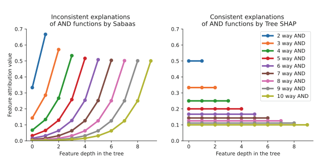
Left Panel (CFC/Saabas Values):

It shows that the CFC method tends to assign much lower importance to features that are closer to the root of a single tree. This results in an inconsistent attribution where even equally relevant features are given unequal credit.

Right Panel (SHAP Values):

In contrast, Tree SHAP distributes credit more evenly among all features involved in the AND function. This consistency highlights the advantage of SHAP in providing fair local explanations.

Takeaways of Figure 4 in the Paper

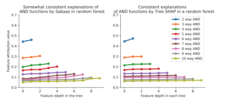
In the ensemble setting, the discrepancies observed in Figure 3 between CFC and SHAP are markedly reduced. The inherent randomness and averaging across trees in the ensemble largely neutralize the bias of CFCs, causing the inconsistency in attributing feature importance (based on tree depth) to almost disappear.

Takeaways of Figure 7 in the Paper

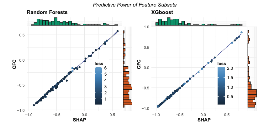
Left Panel (Random Forests):

It shows that the global importance scores calculated via both methods are highly correlated with the model loss across various classification datasets, indicating that they effectively capture the predictive information.

Right Panel (XGBoost):

Similarly, for XGBoost, the correlations are nearly identical—though this panel excludes regression tasks. This consistency suggests that the simpler CFC scores are, on a global level, as reliable as SHAP values for estimating the predictive power of feature subsets.

Conclusion

In summary, this blog reviewed two popular explainable scoring methods for ML models—SHAP values and Conditional Feature Contributions (CFCs). While SHAP provides strong theoretical underpinnings and consistent local explanations by averaging feature contributions over all orderings, it can be computationally heavy for high-dimensional data. CFCs, on the other hand, offer an efficient and intuitive alternative based on the tree’s decision path; however, they may suffer from local biases in single trees. Fortunately, when applied to randomized tree ensembles, these local inconsistencies diminish, and global CFC scores become nearly indistinguishable from SHAP values. This finding underscores the potential of using computationally efficient methods like CFC as reliable approximations for large-scale, production-level interpretability without compromising accuracy.

By integrating these approaches, researchers and practitioners can achieve transparent and reliable explanations, fostering trust in machine learning models across various applications.