German English Translator
Dingyi Lai / February 2022
Machine Translation, an application of Seq2Seq Model
Language modeling enables us to predict the next word/charactor based on previous words/character. Machine translation can be viewed as such a prediction used to generate text. One generalized benefits from this kind of prediction task is, knowledge in language model could be used for other NLP task, e.g. machine translation.
The formal definition of machine translation could be task of translating a sentence x from one language (the source language) to a sentence y in another language (the target language). Although there are many parallel corporas building such a model, such as Europarl [Koehn, 2005] (European Parliament speeches translated into 28 EU languages), MultiUN [Eisele and Chen, 2010] (official United Nations documents translated into 6 languages), ParaCrawl [Banon et al., 2020] (translated web pages) etc., tough challenges still exist, like ambiguities and semantic difference between languages.
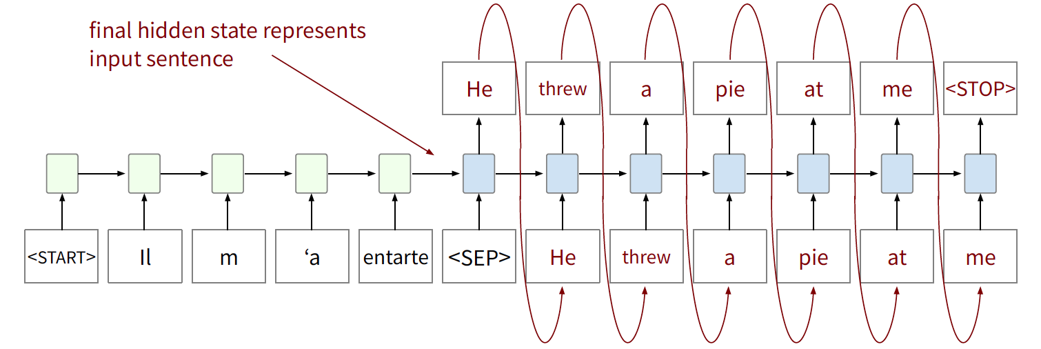
Current machine translation systems apply a sequence-to-sequence neural network architecture (aka seq2seq). It involves two networks (RNNs or transformers):
- one encoder that reads the source text
- (green) only learns to predict a final encoder hidden state
- produces hidden state that is input to decoder
- one decoder that predicts the target text:
- (blue) trained with a language modeling objective, conditioned on final encoder state
- step by step and use previous predictions as input into next step

While being trained, loss is computed for the task of next symbol prediction on the task language sentence. Since decoder RNN is conditioned on output of encoder RNN, the gradient is backpropagated and the entire network is learnt “end-to-end”.
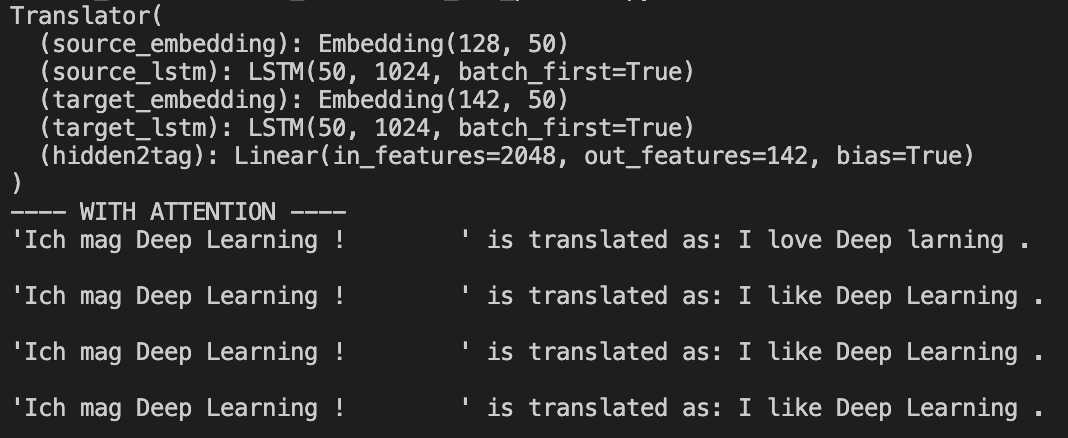
Codes for model with parameters assigning multi-layer, attention, beam search decoding in this repo.
Codes for training are in this repo.
Results with attention could be test in this repo, while without attention in this repo.
Some sample results are like the following.
- with attention

- without attention

Architecture Improvements
Teacher Forcing Ratio
Teacher forcing means that loss is computed at each time step for “gold” input. During training, teacher forcing can be randomly deactivated for a percentage of decoder steps in which predictions instead of gold input are used.

Multi-layer RNNs
In multi-layer RNNs, each layer is an independent RNN cell that takes as input the output of the previous layer. Normally, lower RNNs compute lower-level features and higher RNNs compute higher-level features

In practice, high-performing RNNs for machine translation are usually multi-layer (but arenʼt as deep as convolutional or feed-forward networks). For instance, for Neural Machine Translation [Britz et al., 2017], 2 to 4 layers is the best for the encoder RNN, and 4 layers is the best for the decoder RNN. Obviously, it is often difficult to train deeper RNNs. Skip-connections or other tricks are required while doing so. While for transformer-based networks, they are usually deeper, like 12 or 24 layers, and they have a lot of skipping-like connections.
Different Decoding Approaches
Random Sampling from Multinomial Distribution
Greedy Decoding (i.e. beam search with \(k = 1\))
Greedy decoding generates (or “decodes”) the target sentence by taking argmax on each step of the decoder (take most probable word on each step). It decodes until the model produces a <STOP> token. But the biggist problem is that it has no way to undo decisions, which is desirable in case of ‘temporary false positive’.
Exhaustive Search Decoding (i.e. beam search with \(k = V\))
In exhaustive search decoding, all possible sequences are tried to be computed. This means that on each step \(t\) of the decoder, weʼre tracking \(V \times t\) possible partial translations, where \(V\) is vocabulary size. However, its complexity \(O(VT)\) is far too expensive.
Beam Search Decoding
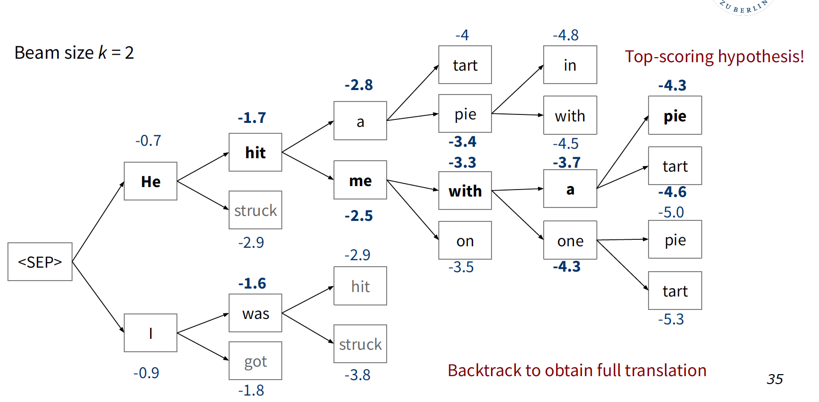
On each step of decoder, keep track of the \(k\) most probable partial translations (which we call hypotheses), where \(k\) is the beam size (in practice around 5 to 10). Although it’s not guaranteed to find optimal solution, it’s still much more efficient than exhaustive search.
The beam search formula is as below:

One of the decoding example would be:

Different hypotheses may produce <STOP> tokens on different time steps. When a hypothesis produces <END>, that hypothesis is complete and placed aside. Other hypotheses via beam search are kept being explored.
Usually we continue beam search until:
- We reach timestep T (where T is some pre-defined cutoff)
- We have at least n completed hypotheses (where n is pre-defined cutoff)
- Normalized by length to fix the problem of ‘longer hypotheses have lower scores’
Attention
Since encoding of the source sentence is a single vector representation (last hidden state), it needs to capture all information about the source sentence when we use RNN cells. Attention provides a solution to the information bottleneck problem. On each step of the decoder, use direct connection to the encoder to focus on a particular part of the source sequence.