home..

Spline Regression

Dingyi Lai / February 2025

Spline regression is a flexible, powerful tool for modeling non‐linear relationships between a response and one or more predictors. Since I am conducting a simulation study involving the calculation of some statistics from a spline regression, I am more than happy trying to introduce the basic idea of spline regression and the relationships among its key parameters. I’ll give an example in both R and Python for better illustration.

What is the basis?

In linear algebra, the most straightforward example of the basis for any vector described as a pair number, which means it starts from \((0,0)\), are the coordinates in the \(xy\)-coordinate system. Some detailed vivid illustrations can be found in the fantastic blog along with its video by 3B1B. More precisely, a basis of a vector space can be defined as a set, \(V\), of elements of the space such that there exist a unique linear combination of elements of \(V\) that is able to express any element of the space.

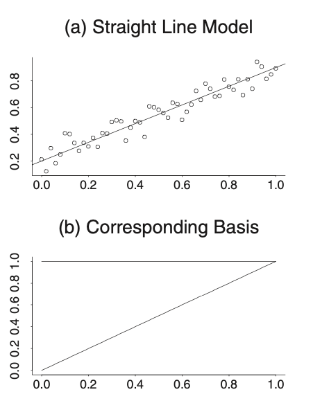
For example, in a linear regression model \(y = \beta_0 + \beta_1 x+ error\), the basis functions are 1 and x. Hence, \(\{1, x\}\) can be viewed as a basis for the vector space in \(x\) for all linear polynomials. It can be illustrated by the following figure:

Conceptual table — Figure 1: The simple linear regression model

Next, consider the nonlinear regression model such as \(y = \beta_0 + \beta_1 x + \beta_2 x^2 + error\):

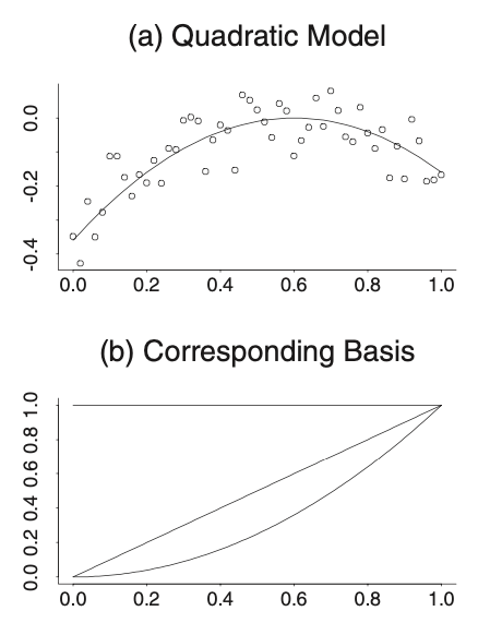
where the basis is obviously \(\{1, x, x^2\}\)

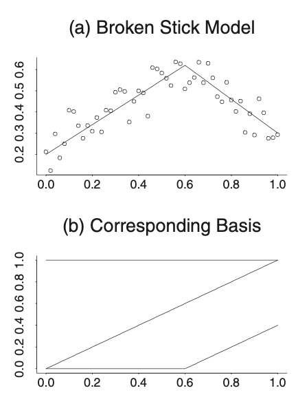
When it’s extended to more complex model like the broken stick model, the indicator function such as \((x-0.6)_{+}\) needs to be included in the basis, as the sloped lines are connected in a stiff manner at \(x=0.6\). Note that this indicator function mean that if \(x-0.6\) is positive, then it indicates itself; otherwise, it’s equal to 0.

Moreover, more indicator functions are included when the right-hand half has more intricate structure:

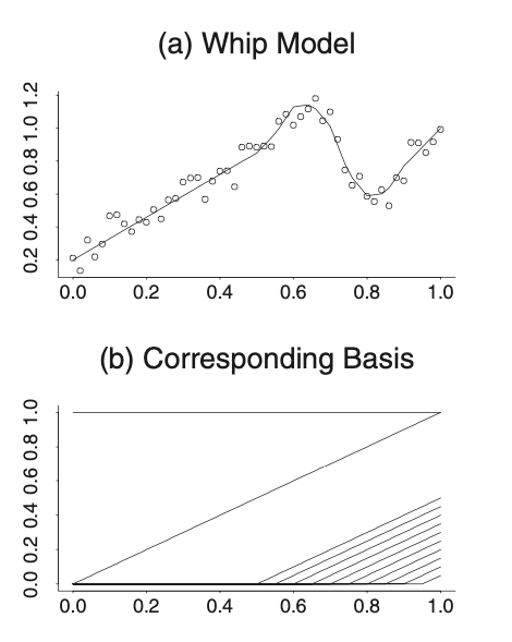
And its basis can be written as:

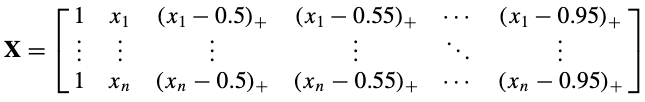
The turning point \(\kappa\) in the indicator \((x-\kappa)_{+}\) is called knot, which leads to the introduction of splines below.

What Are Splines?

Splines are piecewise polynomial functions that are smoothly connected at points knots similar to the above. Instead of forcing a single polynomial to fit the entire dataset—which can lead to underfitting or overfitting—spline regression fits separate polynomial segments between knots. For example, \((x-0.6)_{+}\) can be called as a linear spline basis function, where its knot is at 0.6 and the function itself is called a spline.

Another great idea to think of spline is to imagine the connected scatterplots for the cartoon figures that you draw in your childhood. You can connect the dots bluntly:

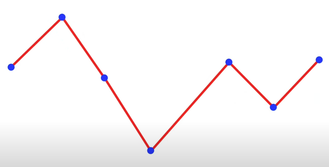
Or you can connect them in a smooth way:

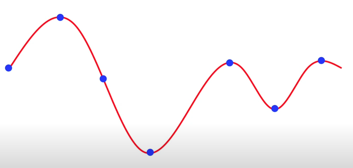
There are mainly three ways to decide the smoothness of the overall curve – The number of knots, the type of splines and the constraints predefined.

Number of knots and its Relationship to Degrees of Freedom

Number of Knots: As illustrated in the former section, the more knots there are, the more detailed it is when the line fit the data. Given the number of knots \(K\) , there are \(2^K\) possible models for automatic knot selection, if you consider including or excluding each candicate independently.
Degrees of Freedom (DF): In the context of spline regression, the degrees of freedom refer to the number of independent parameters estimated. More knots mean more basis functions and, hence, higher degrees of freedom (more flexibility) but also a higher risk of overfitting.
Relationship: For a spline of degree \(p\) with \(K\) interior knots (assuming knots are fixed), the DF is \(K + p + 1\) if intercept is included

Type of splines

Besides the number of knots, the smoothness constraints (usually continuity of the function and some of its derivatives) at the knots restrict their influence, thus ensuring that the overall curve is smooth.

Accordingly, there are several types of splines:

Linear spline is equivalent to the vanilla connected scatterplot
Quadratic spline bases has a continuous first derivative

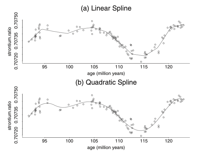
Apparently, the spline function with the degree of the piecewise polynomial being \(p\) has \(p-1\) continuous derivatives. The higher the \(p\) is, the smoother the estimated line.

All the spline functions that I’ve discussed so far is called the truncated power functions, with its basis being:

\[1,\, x,\, \ldots,\, x^p,\quad (x - \kappa_1)_+^p,\ \ldots,\ (x - \kappa_K)_+^p,\]

which is known as the truncated power basis of degree \(p\). The \(p\)-th-degree spline is

\[f(x) \;=\; \beta_0 \;+\; \beta_1\,x \;+\; \cdots \;+\; \beta_p\,x^p \;+\; \sum_{k=1}^{K} \beta_{pk}\,\bigl(x - \kappa_k\bigr)_+^p.\]

However, there are other types of splines that has equivalent bases with more stable numerical properties such as B-spline basis.

B splines is equivalent to the truncated power basis of the same degree in the sense that they span the same set of functions. By span it means the set of all possible linear combinations of the basis functions.
Natural cubic splines are cubic splines that impose additional boundary constraints so that the function is linear outside the outermost knots. This helps avoid the wild oscillations that can occur at the boundaries. Natural splines thus have fewer degrees of freedom than a regular cubic spline with the same knots, because of these boundary constraints.
Radial basis functions (RBF) are commonly used in higher-dimensional settings. An RBF spline typically depends on the distance between the predictor variable (often in multiple dimensions) and the knot location. A popular example is the Gaussian RBF \(\exp\bigl(-\gamma \lVert x - \kappa \rVert^2\bigr)\). These are especially powerful for smoothing in spatial or multi-dimensional data, but they also come with their own complexities in selecting parameters (like \(\gamma\)).

Penalized Spline Regression

Apart from defining the number of knots and the type of splines, penalizing the spline regression is another method to control the smoothness.

Consider a spline model with \(K\) knots, \(\beta\) in the following formula, which is a matrix of the coefficients of the knots, has \(K\) elements. The constraints on \(\beta\) given some number \(\lambda \ge 0\) leads to the solution:

\[\widehat{\beta} = \bigl(X^\mathsf{T}X + \lambda^2 D\bigr)^{-1} X^\mathsf{T}y.\]

The term \(\lambda^2 \beta^\mathsf{T} D \beta\) is called a roughness penalty because it penalizes fits that are too rough, thus yielding a smoother result. The amount of smoothing is controlled by \(\lambda\), which is therefore usually referred to as a smoothing parameter.

The fitted values for a penalized spline regression are then given by:

\[\widehat{y} \;=\; X \,\bigl(X^\mathsf{T}X + \lambda^2 D\bigr)^{-1} X^\mathsf{T}y.\]

An Example: Simulating Non-Linear Data

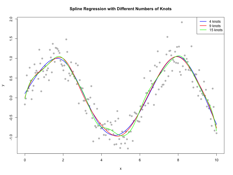
Let’s simulate a dataset where the true relationship is non-linear (say, a sine curve with some noise) and fit spline regressions with different numbers of knots to see how the degrees of freedom change.

Implementation in R

Below is an R code example using the splines package. We’ll simulate data, fit models with varying numbers of knots, and extract the effective degrees of freedom.

# Load necessary library
library(splines)
set.seed(123)

# Simulate data: y = sin(x) + noise
n <- 200
x <- seq(0, 10, length.out = n)
y <- sin(x) + rnorm(n, sd = 0.3)
data <- data.frame(x, y)

write.csv(data, "_data/spline.csv", row.names = FALSE)

# Fit spline regression with different numbers of knots
# Model 1: 3 interior knots
model1 <- lm(y ~ bs(x, df = 7), data = data)
knots1 <- attr(bs(x, df = 7), "knots")

# Model 2: 5 interior knots
model2 <- lm(y ~ bs(x, df = 12), data = data)
knots2 <- attr(bs(x, df = 12), "knots")

# Model 3: 7 interior knots
model3 <- lm(y ~ bs(x, df=18), data = data)
knots3 <- attr(bs(x, df = 18), "knots")

# Print degrees of freedom
cat("Number of knots for cubic spline model with df=4:", length(knots1), "\n")
cat("Number of knots for cubic spline model with df=10:", length(knots2), "\n")
cat("Number of knots for cubic spline model with df=16:", length(knots3), "\n")

# Plot the data and fitted curves
# file.exists("_images")
png("_images/[SR]spline_regression_R.png", width = 800, height = 600)
plot(x, y, main = "Spline Regression with Different Numbers of Knots", 
     pch = 19, col = "grey", xlab = "x", ylab = "y")
lines(x, predict(model1, newdata = data), col = "blue", lwd = 2)
lines(x, predict(model2, newdata = data), col = "red", lwd = 2)
lines(x, predict(model3, newdata = data), col = "green", lwd = 2)
legend("topright", legend = c("4 knots", "9 knots", "15 knots"),
       col = c("blue", "red", "green"), lwd = 2)
dev.off()

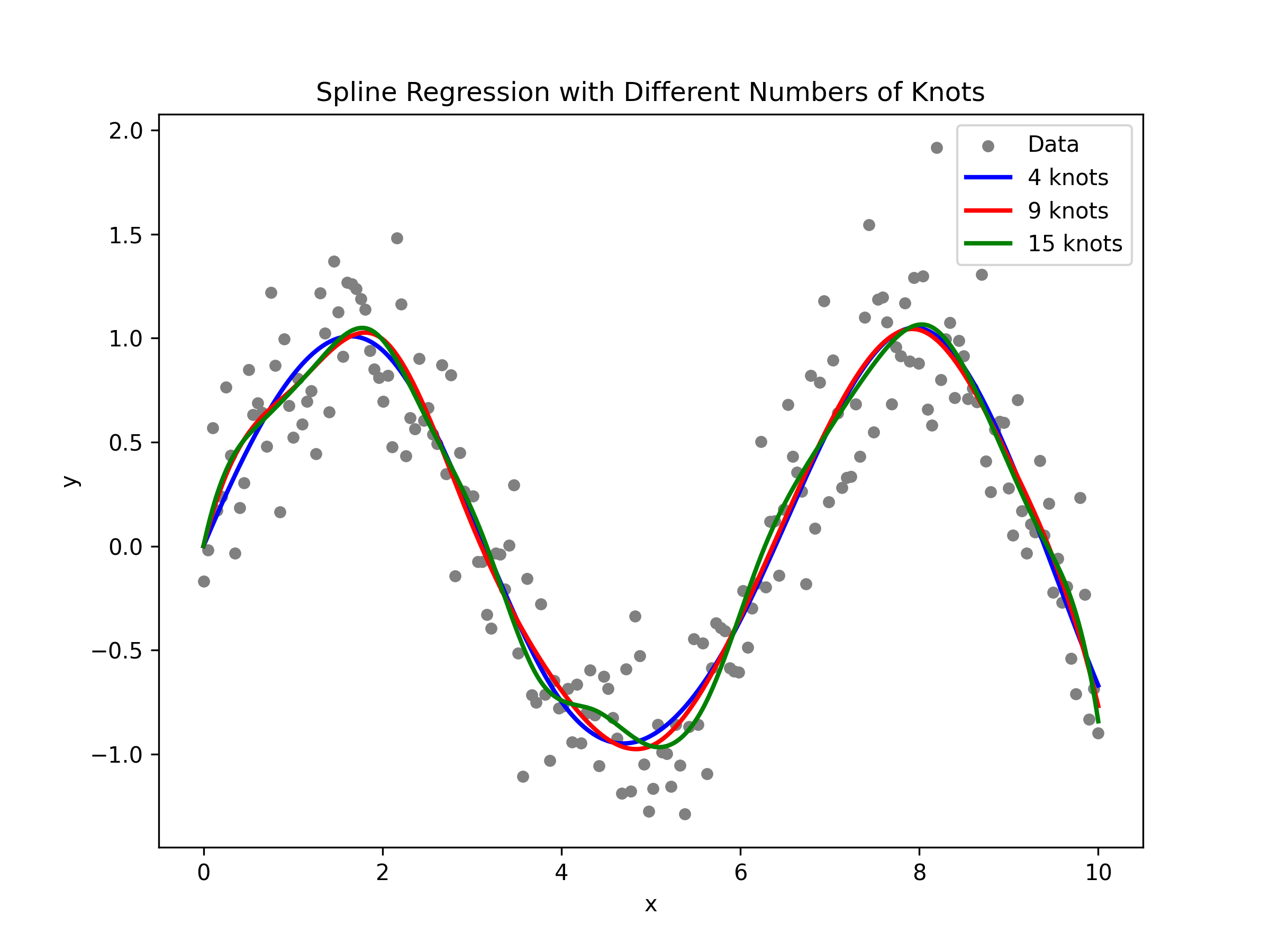
Implementation in Python

Now let’s perform a similar analysis in Python using patsy for spline basis creation and statsmodels for fitting the regression model.

import numpy as np
import pandas as pd
import matplotlib.pyplot as plt
from statsmodels.gam.api import BSplines
import statsmodels.api as sm

# Set random seed for reproducibility
np.random.seed(123)

# Simulate data: y = sin(x) + noise
n = 200
# Read the data from the CSV file
data = pd.read_csv("../_data/spline.csv")

# If you need to extract the 'x' and 'y' values:
x = data['x'].values
y = data['y'].values
# statsmodels expects exogenous variables as a 2D array:
x_2d = x[:, None]

# ---- Model 1: Using 4 degrees of freedom ----
# In this context, we set df=[4] which mimics R's bs(x, df=4) for a single predictor.
bs1 = BSplines(x_2d, df=[8], degree=[3])
# Fit OLS using the spline basis
model1 = sm.OLS(y, bs1.transform(x_2d)).fit()
# Extract knots; bs1.knots is a list (one array per predictor)
knots1 = bs1.dim_basis - bs1.degrees[0]
print("Number of knots for cubic spline model with df=4:", knots1)

# ---- Model 2: Using 10 degrees of freedom ----
bs2 = BSplines(x_2d, df=[13], degree=[3])
model2 = sm.OLS(y, bs2.transform(x_2d)).fit()
knots2 = bs2.dim_basis - bs2.degrees[0]
print("Number of knots for cubic spline model with df=10:", knots2)

# ---- Model 3: Using 16 degrees of freedom ----
bs3 = BSplines(x_2d, df=[19], degree=[3])
model3 = sm.OLS(y, bs3.transform(x_2d)).fit()
knots3 = bs3.dim_basis - bs3.degrees[0]
print("Number of knots for cubic spline model with df=16:", knots3)

# Create a fine grid for prediction
x_pred = np.linspace(0, 10, 500)[:, None]

# Generate predictions from the three models
y_pred1 = model1.predict(bs1.transform(x_pred))
y_pred2 = model2.predict(bs2.transform(x_pred))
y_pred3 = model3.predict(bs3.transform(x_pred))

# Plot the data and fitted curves
plt.figure(figsize=(8, 6))
plt.scatter(x, y, color="grey", s=20, label="Data")
plt.plot(x_pred.flatten(), y_pred1, color="blue", lw=2, label="4 knots")
plt.plot(x_pred.flatten(), y_pred2, color="red", lw=2, label="9 knots")
plt.plot(x_pred.flatten(), y_pred3, color="green", lw=2, label="15 knots")
plt.title("Spline Regression with Different Numbers of Knots")
plt.xlabel("x")
plt.ylabel("y")
plt.legend(loc="upper right")
# Save the plot to a file (ensure that the directory '_images' exists)
plt.savefig("../_images/[SR]spline_regression_python.png", dpi=300)
plt.show()

Comparison: R vs. Python

R
- df = 7 & cubic -> 4 knots (7 = 4+3)
- df = 12 & cubic -> 9 knots (12 = 9+3)
- df = 18 & cubic -> 15 knots (18 = 15+3)
Python
- df = 5 & cubic -> 4 knots (4 = 5-1)
- df = 10 & cubic -> 9 knots (9 = 10-1)
- df = 16 & cubic -> 15 knots (15 = 16-1)
Definition from different versions:
- df in R from library(splines): df degrees of freedom; one can specify df rather than knots; bs() then chooses df-degree (minus one if there is an intercept) knots at suitable quantiles of x (which will ignore missing values). The default, NULL, takes the number of inner knots as length(knots). If that is zero as per default, that corresponds to df = degree - intercept
- df in Python from from statsmodels.gam.api import BSplines number of basis functions or degrees of freedom; should be equal in length to the number of columns of x; may be an integer if x has one column or is 1-D.
- df in Python from from sddr.splines import spline, Spline Number of degrees of freedom (equals the number of columns in s.basis) because Intercept is set to be True by default

Conclusion

Spline regression is a versatile method for modeling complex, non-linear relationships. The number of knots, the type of splines and possible penalty can be used to control the flexibility of your model. By comparing implementations in R and Python, we see that the relationship between the parameter df and the number of knots are different in different version.

Feel free to experiment with the provided code examples to better understand how the choice of knots affects model flexibility. If you have any questions or insights, share your thoughts in the comments!

Happy modeling!

Reference:

Ruppert, D., Wand, M.P. and Carroll, R.J. (2003) Semiparametric Regression. Cambridge: Cambridge University Press (Cambridge Series in Statistical and Probabilistic Mathematics).
https://www.3blue1brown.com/lessons/span
https://www.youtube.com/watch?v=YMl25iCCRew
https://www.rdocumentation.org/packages/splines/versions/3.6.2/topics/bs
https://www.statsmodels.org/dev/generated/statsmodels.gam.smooth_basis.BSplines.html
https://github.com/HelmholtzAI-Consultants-Munich/PySDDR/tree/master/sddr
https://www.kirenz.com/blog/posts/2021-12-06-regression-splines-in-python/